4. Inputs and Outputs

The ufs-weather-model can be configured as one of several applications, from a single component atmosphere model to a fully coupled model with multiple earth system components (atmosphere, ocean, sea-ice and mediator). Currently the supported configurations are:

Table 4.1 Supported ufs-weather-model applications

App name	Description
ATM	Standalone UFSAtm
ATMW	UFSAtm coupled to WW3
ATMAERO	UFSAtm coupled to GOCART
S2S	Coupled UFSATM-MOM6-CICE6-CMEPS
S2SW	Coupled UFSATM-MOM6-CICE6-WW3-CMEPS
NG-GODAS	Coupled CDEPS-DATM-MOM6-CICE6-CMEPS
HAFS	Coupled UFSATM-HYCOM-CMEPS
HAFSW	Coupled UFSATM-HYCOM-WW3-CMEPS
HAFS-ALL	Coupled CDEPS-UFSATM-HYCOM-WW3-CMEPS

This chapter describes the input and output files needed for executing the model in the various supported configurations.

4.1. Input files

There are three types of files needed to execute a run: static datasets (fix files containing climatological information), files that depend on grid resolution, initial and boundary conditions, and model configuration files (such as namelists).

4.1.1. UFSAtm

4.1.1.1. Static datasets (i.e., fix files)

The static input files for global configurations are listed and described in Table 4.2. Similar files are used for a regional grid but are grid specific and generated by pre-processing utilities.

Table 4.2 Fix files containing climatological information

Filename	Description
aerosol.dat	External aerosols data file
CFSR.SEAICE.1982.2012.monthly.clim.grb	CFS reanalysis of monthly sea ice climatology
co2historicaldata_YYYY.txt	Monthly CO2 in PPMV data for year YYYY
global_albedo4.1x1.grb	Four albedo fields for seasonal mean climatology: 2 for strong zenith angle dependent (visible and near IR) and 2 for weak zenith angle dependent
global_glacier.2x2.grb	Glacier points, permanent/extreme features
global_h2oprdlos.f77	Coefficients for the parameterization of photochemical production and loss of water (H2O)
global_maxice.2x2.grb	Maximum ice extent, permanent/extreme features
global_mxsnoalb.uariz.t126.384.190.rg.grb	Climatological maximum snow albedo
global_o3prdlos.f77	Monthly mean ozone coefficients
global_shdmax.0.144x0.144.grb	Climatological maximum vegetation cover
global_shdmin.0.144x0.144.grb	Climatological minimum vegetation cover
global_slope.1x1.grb	Climatological slope type
global_snoclim.1.875.grb	Climatological snow depth
global_snowfree_albedo.bosu.t126.384.190.rg.grb	Climatological snowfree albedo
global_soilmgldas.t126.384.190.grb	Climatological soil moisture
global_soiltype.statsgo.t126.384.190.rg.grb	Soil type from the STATSGO dataset
global_tg3clim.2.6x1.5.grb	Climatological deep soil temperature
global_vegfrac.0.144.decpercent.grb	Climatological vegetation fraction
global_vegtype.igbp.t126.384.190.rg.grb	Climatological vegetation type
global_zorclim.1x1.grb	Climatological surface roughness
RTGSST.1982.2012.monthly.clim.grb	Monthly, climatological, real-time global sea surface temperature
seaice_newland.grb	High resolution land mask
sfc_emissivity_idx.txt	External surface emissivity data table
solarconstant_noaa_an.txt	External solar constant data table

4.1.1.2. Grid description and initial condition files

The input files containing grid information and the initial conditions for global configurations are listed and described in Table 4.3. The input files for a limited area model (LAM) configuration including grid information and initial and lateral boundary conditions are listed and described in Table 4.4. Note that the regional grid is referred to as Tile 7 here, and are generated by several pre-processing utilities.

Table 4.3 Input files containing grid information and initial conditions for global configurations

Filename	Description	Date-dependent
Cxx_grid.tile[1-6].nc	Cxx grid information for tiles 1-6, where ‘xx’ is the grid number
gfs_ctrl.nc	NCEP NGGPS tracers, ak, and bk	✔
gfs_data.tile[1-6].nc	Initial condition fields (ps, u, v, u, z, t, q, O3). May include spfo3, spfo, spf02 if multiple gases are used	✔
oro_data.tile[1-6].nc	Model terrain (topographic/orographic information) for grid tiles 1-6
sfc_ctrl.nc	Control parameters for surface input: forecast hour, date, number of soil levels
sfc_data.tile[1-6].nc	Surface properties for grid tiles 1-6	✔

Table 4.4 Regional input files containing grid information and initial and lateral boundary conditions for regional configurations

Filename	Description	Date-dependent
Cxx_grid.tile7.nc	Cxx grid information for tile 7, where ‘xx’ is the grid number
gfs_ctrl.nc	NCEP NGGPS tracers, ak, and bk	✔
gfs_bndy.tile7.HHH.nc	Lateral boundary conditions at hour HHH	✔
gfs_data.tile7.nc	Initial condition fields (ps, u, v, u, z, t, q, O3). May include spfo3, spfo, spf02 if multiple gases are used	✔
oro_data.tile7.nc	Model terrain (topographic/orographic information) for grid tile 7
sfc_ctrl.nc	Control parameters for surface input: forecast hour, date, number of soil levels
sfc_data.tile7.nc	Surface properties for grid tile 7	✔

4.1.2. MOM6

4.1.2.1. Static datasets (i.e., fix files)

The static input files for global configurations are listed and described in Table 4.5.

Table 4.5 Fix files containing climatological information

Filename	Description	Used in resolution
runoff.daitren.clim.1440x1080.v20180328.nc	climatological runoff	0.25
runoff.daitren.clim.720x576.v20180328.nc	climatological runoff	0.50
seawifs-clim-1997-2010.1440x1080.v20180328.nc	climatological chlorophyll concentration in sea water	0.25
seawifs-clim-1997-2010.720x576.v20180328.nc	climatological chlorophyll concentration in sea water	0.50
seawifs_1998-2006_smoothed_2X.nc	climatological chlorophyll concentration in sea water	1.00
tidal_amplitude.v20140616.nc	climatological tide amplitude	0.25
tidal_amplitude.nc	climatological tide amplitude	0.50, 1.00
geothermal_davies2013_v1.nc	climatological geothermal heat flow	0.50, 0.25
KH_background_2d.nc	climatological 2-d background harmonic viscosities	1.00

4.1.2.2. Grid description and initial condition files

The input files containing grid information and the initial conditions for global configurations are listed and described in Table 4.6.

Table 4.6 Input files containing grid information and initial conditions for global configurations

Filename	Description	Valid RES options	Date-dependent
ocean_hgrid.nc	horizonal grid information	1.00, 0.50, 0.25
ocean_mosaic.nc	specify horizonal starting and ending points index	1.00, 0.50, 0.25
ocean_topog.nc	ocean topography	1.00, 0.50, 0.25
ocean_mask.nc	lans/sea mask	1.00, 0.50, 0.25
hycom1_75_800m.nc	vertical coordinate level thickness	1.00, 0.50, 0.25
layer_coord.nc	vertical layer target potential density	1.00, 0.50, 0.25
All_edits.nc	specify grid points where topography are manually modified to adjust throughflow strength for narrow channels	0.25
topo_edits_011818.nc	specify grid points where topography are manually modified to adjust throughflow strength for narrow channels	1.00
MOM_channels_global_025	specifies restricted channel widths	0.50, 0.25
MOM_channel_SPEAR	specifies restricted channel widths	1.00
interpolate_zgrid_40L.nc	specify target depth for output	1.00, 0.50, 0.25
MOM.res*nc	ocean initial conditions (from CPC ocean DA)	0.25	✔
MOM6_IC_TS.nc	ocean temperature and salinity initial conditions (from CFSR)	1.00, 0.50, 0.25	✔

4.1.3. HYCOM

4.1.3.1. Static datasets (i.e., fix files)

Static input files have been created for several regional domains. These domains are listed and described in Table 4.7.

Table 4.7 The following table describes each domain identifier.

Identifier	Description
hat10	Hurricane North Atlantic (1/12 degree)
hep20	Hurricane Eastern North Pacific (1/12 degree)
hwp30	Hurricane Western North Pacific (1/12 degree)
hcp70	Hurricane Central North Pacific (1/12 degree)

Static input files are listed and described in Table 4.8. Several datasets contain both dot-a (.a) and dot-b (.b) files. Dot-a files contain data written as 32-bit IEEE real values (idm*jdm) and dot-b files contain plain text metadata for each field in the dot-a file.

Table 4.8 Fix files containing climatological information

Filename	Description	Domain
blkdat.input	Model input parameters
patch.input	Tile description
ports.input	Open boundary cells
forcing.chl.(a,b)	Chlorophyll (monthly climatology)	hat10, hep20, hwp30, hcp70
forcing.rivers.(a,b)	River discharge (monthly climatology)	hat10, hep20, hwp30, hcp70
iso.sigma.(a,b)	Fixed sigma thickness	hat10, hep20, hwp30, hcp70
regional.depth.(a,b)	Total depth of ocean	hat10, hep20, hwp30, hcp70
regional.grid.(a,b)	Grid information for HYCOM “C” grid	hat10, hep20, hwp30, hcp70
relax.rmu.(a,b)	Open boundary nudging value	hat10, hep20, hwp30, hcp70
relax.ssh.(a,b)	Surface height nudging value (monthly climatology)	hat10, hep20, hwp30, hcp70
tbaric.(a,b)	Thermobaricity correction	hat10, hep20, hwp30, hcp70
thkdf4.(a,b)	Diffusion velocity (m/s) for Laplacian thickness diffusivity	hat10, hep20, hwp30, hcp70
veldf2.(a,b)	Diffusion velocity (m/s) for biharmonic momentum dissipation	hat10, hep20, hwp30, hcp70
veldf4.(a,b)	Diffusion velocity (m/s) for Laplacian momentum dissipation	hat10, hep20, hwp30, hcp70

4.1.3.2. Grid description and initial condition files

The input files containing time dependent configuration and forcing data are listed and described in Table 4.9. These files are generated for specific regional domains, see Table 4.7, during ocean prep. When uncoupled, the the forcing data drives the ocean model. When coupled, the forcing data is used to fill unmapped grid cells. Several datasets contain both dot-a (.a) and dot-b (.b) files. Dot-a files contain data written as 32-bit IEEE real values (idm*jdm) and dot-b files contain plain text metadata for each field in the dot-a file.

Table 4.9 Input files containing grid information, initial conditions, and forcing data for regional configurations.

Filename	Description	Domain	Date-dependent
limits	Model begin and end time (since HYCOM epoch)		✔
forcing.airtmp.(a,b)	GFS forcing data for 2m air temperature	hat10, hep20, hwp30, hcp70	✔
forcing.mslprs.(a,b)	GFS forcing data for mean sea level pressure (symlink)	hat10, hep20, hwp30, hcp70	✔
forcing.precip.(a,b)	GFS forcing data for precipitation rate	hat10, hep20, hwp30, hcp70	✔
forcing.presur.(a,b)	GFS forcing data for mean sea level pressure	hat10, hep20, hwp30, hcp70	✔
forcing.radflx.(a,b)	GFS forcing data for total radiation flux	hat10, hep20, hwp30, hcp70	✔
forcing.shwflx.(a,b)	GFS forcing data for net downward shortwave radiation flux	hat10, hep20, hwp30, hcp70	✔
forcing.surtmp.(a,b)	GFS forcing data for surface temperature	hat10, hep20, hwp30, hcp70	✔
forcing.tauewd.(a,b)	GFS forcing data for eastward momentum flux	hat10, hep20, hwp30, hcp70	✔
forcing.taunwd.(a,b)	GFS forcing data for northward momentum flux	hat10, hep20, hwp30, hcp70	✔
forcing.vapmix.(a,b)	GFS forcing data for 2m vapor mixing ratio	hat10, hep20, hwp30, hcp70	✔
forcing.wndspd.(a,b)	GFS forcing data for 10m wind speed	hat10, hep20, hwp30, hcp70	✔
restart_in.(a,b)	Restart file for ocean state variables	hat10, hep20, hwp30, hcp70	✔

4.1.4. CICE6

4.1.4.1. Static datasets (i.e., fix files)

No fix files are required for CICE6

4.1.4.2. Grid description and initial condition files

The input files containing grid information and the initial conditions for global configurations are listed and described in Table 4.10.

Table 4.10 Input files containing grid information and initial conditions for global configurations

Filename	Description	Valid RES options	Date-dependent
cice_model_RES.res_YYYYMMDDHH.nc	cice model IC or restart file	1.00, 0.50, 0.25	✔
grid_cice_NEMS_mxRES.nc	cice model grid at resolution RES	100, 050, 025
kmtu_cice_NEMS_mxRES.nc	cice model land mask at resolution RES	100, 050, 025

4.1.5. WW3

4.1.5.1. Static datasets (i.e., fix files)

No fix files are required for WW3

4.1.5.2. Grid description and initial condition files

The files for global configurations are listed and described in Table 4.11 for GFSv16 setup and Table 4.12 for single grid configurations. The model definitions for wave grid(s) including spectral and directional resolutions, time steps, numerical scheme and parallelization algorithm, the physics parameters, boundary conditions and grid definitions are stored in binary mod_def files. The aforementioned parameters are defined in ww3_grid.inp.<grd> and the ww3_grid executables generates the binary mod_def.<grd> files.

The WW3 version number in mod_def.<grd> files must be consistent with version of the code in ufs-weather-model. createmoddefs/creategridfiles.sh can be used in order to generate the mod_def.<grd> files, using ww3_grid.inp.<grd>, using the WW3 version in ufs-weather-model. In order to do it, the path to the location of the ufs-weather-model (UFSMODELDIR), the path to generated mod_def.<grd> outputs (OUTDIR), the path to input ww3_grid.inp.<grd> files (SRCDIR) and the path to the working directory for log files (WORKDIR) should be defined.

Table 4.11 Input files containing grid information and conservative remapping for global configurations (GFSv16 Wave)

Filename	Description	Spatial Resolution	nFreq	nDir
mod_def.aoc_9km	Antarctic Ocean PolarStereo [50N 90N]	9km	50	36
mod_def.gnh_10m	Global mid core [15S 52N]	10 min	50	36
mod_def.gsh_15m	southern ocean [79.5S 10.5S]	15 min	50	36
mod_def.glo_15mxt	Global 1/4 extended grid [90S 90S]	15 min	36	24
mod_def.points	GFSv16-wave spectral grid point output	na	na	na
rmp_src_to_dst_conserv_002_001.nc	Conservative remapping gsh_15m to gnh_10m	na	na	na
rmp_src_to_dst_conserv_003_001.nc	Conservative remapping aoc_9km to gnh_10m	na	na	na

Table 4.12 Input grid information for single global/regional configurations

Filename	Description	Spatial Resolution	nFreq	nDir
mod_def.ant_9km	Regional polar stereo antarctic grid [90S 50S]	9km	36	24
mod_def.glo_10m	Global grid [80S 80N]	10 min	36	24
mod_def.glo_30m	Global grid [80S 80N]	30 min	36	36
mod_def.glo_1deg	Global grid [85S 85N]	1 degree	25	24
mod_def.glo_2deg	Global grid [85S 85N]	2 degree	20	18
mod_def.glo_5deg	Global grid [85S 85N]	5 degree	18	12
mod_def.glo_gwes_30m	Global NAWES 30 min wave grid [80S 80N]	30 min	36	36
mod_def.natl_6m	Regional North Atlantic Basin [1.5N 45.5N; 98W 8W]	6 min	50	36

Coupled regional configurations require forcing files to fill regions that cannot be interpolated from the atmospheric component. For a list of forcing files used to fill unmapped data points see Table 4.13.

Table 4.13 Forcing information for single regional configurations

Filename	Description	Resolution
wind.natl_6m	Interpolated wind data from GFS	6 min

The model driver input (ww3_multi.inp) includes the input, model and output grids definition, the starting and ending times for the entire model run and output types and intervals. The ww3_multi.inp.IN template is located under tests/parm/ directory. The inputs are described hereinafter:

Table 4.14 Model driver input

NMGRIDS	Number of wave model grids
NFGRIDS	Number of grids defining input fields
FUNIPNT	Flag for using unified point output file.
IOSRV	Output server type
FPNTPROC	Flag for dedicated process for unified point output
FGRDPROC	Flag for grids sharing dedicated output processes

If there are input data grids defined ( NFGRIDS > 0 ) then these grids are defined first (CPLILINE, WINDLINE, ICELINE, CURRLINE). These grids are defined as if they are wave model grids using the file mod_def.<grd>. Each grid is defined on a separate input line with <grd>, with nine input flags identifying $ the presence of 1) water levels 2) currents 3) winds 4) ice $ 5) momentum 6) air density and 7-9) assimilation data.

The UNIPOINTS defines the name of this grid for all point output, which gathers the output spectral grid in a unified point output file.

The WW3GRIDLINE defines actual wave model grids using 13 parameters to be read from a single line in the file for each. It includes (1) its own input grid mod_def.<grd>, (2-10) forcing grid ids, (3) rank number, (12) group number and (13-14) fraction of communicator (processes) used for this grid.

RUN_BEG and RUN_END define the starting and end times, FLAGMASKCOMP and FLAGMASKOUT are flags for masking at printout time (default F F), followed by the gridded and point outputs start time (OUT_BEG), interval (DTFLD and DTPNT) and end time (OUT_END). The restart outputs start time, interval and end time are define by RST_BEG, DTRST, RST_END respectively.

The OUTPARS_WAV defines gridded output fields. The GOFILETYPE, POFILETYPE and RSTTYPE are gridded, point and restart output types respectively.

No initial condition files are required for WW3.

4.1.6. CDEPS

4.1.6.1. Static datasets (i.e., fix files)

No fix files are required for CDEPS

4.1.6.2. Grid description and initial condition files

The input files containing grid information and the time-varying forcing files for global configurations are listed and described in Table 4.15 and Table 4.16.

Data Atmosphere

Table 4.15 Input files containing grid information and forcing files for global configurations

Filename	Description	Date-dependent
cfsr_mesh.nc	ESMF mesh file for CFSR data source
gefs_mesh.nc	ESMF mesh file for GEFS data source
TL639_200618_ESMFmesh.nc	ESMF mesh file for ERA5 data source
cfsr.YYYYMMM.nc	CFSR forcing file for year YYYY and month MM	✔
gefs.YYYYMMM.nc	GEFS forcing file for year YYYY and month MM	✔
ERA5.TL639.YYYY.MM.nc	ERA5 forcing file for year YYYY and month MM	✔

Data Ocean

Table 4.16 Input files containing grid information and forcing files for global configurations

Filename	Description	Date-dependent
TX025_210327_ESMFmesh_py.nc	ESMF mesh file for OISST data source
sst.day.mean.YYYY.nc	OISST forcing file for year YYYY	✔

Table 4.17 Input files containing grid information and forcing files for regional configurations

Filename	Description	Date-dependent
hat10_210129_ESMFmesh_py.nc	ESMF mesh file for MOM6 data source
GHRSST_mesh.nc	ESMF mesh file for GHRSST data source
hycom_YYYYMM_surf_nolev.nc	MOM6 forcing file for year YYYY and month MM	✔
ghrsst_YYYYMMDD.nc	GHRSST forcing file for year YYYY, month MM and day DD	✔

4.1.7. GOCART

4.1.7.1. Static datasets (i.e., fix files)

Todo

GOCART information in progress

The static input files for global configurations are listed and described in Table 4.18.

Table 4.18 Fix files containing climatological information

Filename	Description

4.1.7.2. Grid description and initial condition files

Todo

GOCART information in progress

The input files containing grid information and the initial conditions for global configurations are listed and described in Table 4.19.

Table 4.19 Input files containing grid information and initial conditions for global configurations

Filename	Description	Date-dependent

4.2. Model configuration files

The configuration files used by the UFS Weather Model are listed here and described below:

• diag_table

• field_table

• model_configure

• nems.configure

• suite_[suite_name].xml (used only at build time)

• datm.streams (used by cdeps)

• datm_in (used by cdeps)

• blkdat.input (used by HYCOM)

While the input.nml file is also a configuration file used by the UFS Weather Model, it is described in Section 4.2.9. The run-time configuration of model output fields is controlled by the combination of diag_table and model_configure, and is described in detail in Section 4.3.

4.2.1. diag_table file

There are three sections in file diag_table: Header (Global), File, and Field. These are described below.

Header Description

The Header section must reside in the first two lines of the diag_table file and contain the title and date of the experiment (see example below). The title must be a Fortran character string. The base date is the reference time used for the time units, and must be greater than or equal to the model start time. The base date consists of six space-separated integers in the following format: year month day hour minute second. Here is an example:

20161003.00Z.C96.64bit.non-mono
2016 10 03 00 0 0

File Description

The File Description lines are used to specify the name of the file(s) to which the output will be written. They contain one or more sets of six required and five optional fields (optional fields are denoted by square brackets [ ]). The lines containing File Descriptions can be intermixed with the lines containing Field Descriptions as long as files are defined before fields that are to be written to them. File entries have the following format:

"file_name", output_freq, "output_freq_units", file_format, "time_axis_units", "time_axis_name"
[, new_file_freq, "new_file_freq_units"[, "start_time"[, file_duration, "file_duration_units"]]]

These file line entries are described in Table 4.20.

Table 4.20 Description of the six required and five optional fields used to define output file sampling rates.

File Entry	Variable Type	Description
file_name	CHARACTER(len=128)	Output file name without the trailing “.nc”
output_freq	INTEGER	The period between records in the file_name: > 0 output frequency in output_freq_units. = 0 output frequency every time step (output_freq_units is ignored) =-1 output at end of run only (output_freq_units is ignored)
output_freq_units	CHARACTER(len=10)	The units in which output_freq is given. Valid values are “years”, “months”, “days”, “minutes”, “hours”, or “seconds”.
file_format	INTEGER	Currently only the netCDF file format is supported. = 1 netCDF
time_axis_units	CHARACTER(len=10)	The units to use for the time-axis in the file. Valid values are “years”, “months”, “days”, “minutes”, “hours”, or “seconds”.
time_axis_name	CHARACTER(len=128)	Axis name for the output file time axis. The character string must contain the string ‘time’. (mixed upper and lowercase allowed.)
new_file_freq	INTEGER, OPTIONAL	Frequency for closing the existing file, and creating a new file in new_file_freq_units.
new_file_freq_units	CHARACTER(len=10), OPTIONAL	Time units for creating a new file: either years, months, days, minutes, hours, or seconds. NOTE: If the new_file_freq field is present, then this field must also be present.
start_time	CHARACTER(len=25), OPTIONAL	Time to start the file for the first time. The format of this string is the same as the global date. NOTE: The new_file_freq and the new_file_freq_units fields must be present to use this field.
file_duration	INTEGER, OPTIONAL	How long file should receive data after start time in file_duration_units. This optional field can only be used if the start_time field is present. If this field is absent, then the file duration will be equal to the frequency for creating new files. NOTE: The file_duration_units field must also be present if this field is present.
file_duration_units	CHARACTER(len=10), OPTIONAL	File duration units. Can be either years, months, days, minutes, hours, or seconds. NOTE: If the file_duration field is present, then this field must also be present.

Field Description

The field section of the diag_table specifies the fields to be output at run time. Only fields registered with register_diag_field(), which is an API in the FMS diag_manager routine, can be used in the diag_table.

Registration of diagnostic fields is done using the following syntax

diag_id = register_diag_field(module_name, diag_name, axes, ...)

in file FV3/atmos_cubed_sphere/tools/fv_diagnostics.F90. As an example, the sea level pressure is registered as:

id_slp = register_diag_field (trim(field), 'slp', axes(1:2), &   Time, 'sea-level pressure', 'mb', missing_value=missing_value, range=slprange )

All data written out by diag_manager is controlled via the diag_table. A line in the field section of the diag_table file contains eight variables with the following format:

"module_name", "field_name", "output_name", "file_name", "time_sampling", "reduction_method", "regional_section", packing

These field section entries are described in Table 4.21.

Table 4.21 Description of the eight variables used to define the fields written to the output files.

Field Entry	Variable Type	Description
module_name	CHARACTER(len=128)	Module that contains the field_name variable. (e.g. dynamic, gfs_phys, gfs_sfc)
field_name	CHARACTER(len=128)	The name of the variable as registered in the model.
output_name	CHARACTER(len=128)	Name of the field as written in file_name.
file_name	CHARACTER(len=128)	Name of the file where the field is to be written.
time_sampling	CHARACTER(len=50)	Currently not used. Please use the string “all”.
reduction_method	CHARACTER(len=50)	The data reduction method to perform prior to writing data to disk. Current supported option is .false.. See FMS/diag_manager/diag_table.F90 for more information.
regional_section	CHARACTER(len=50)	Bounds of the regional section to capture. Current supported option is “none”. See FMS/diag_manager/diag_table.F90 for more information.
packing	INTEGER	Fortran number KIND of the data written. Valid values: 1=double precision, 2=float, 4=packed 16-bit integers, 8=packed 1-byte (not tested).

Comments can be added to the diag_table using the hash symbol (#).

A brief example of the diag_table is shown below. “...” denotes where lines have been removed.

 20161003.00Z.C96.64bit.non-mono
 2016 10 03 00 0 0

 "grid_spec",     -1,  "months",   1, "days",  "time"
 "atmos_4xdaily",  6,  "hours",    1, "days",  "time"
 "atmos_static"   -1,  "hours",    1, "hours", "time"
 "fv3_history",    0,  "hours",    1, "hours", "time"
 "fv3_history2d",  0,  "hours",    1, "hours", "time"

 #
 #=======================
 # ATMOSPHERE DIAGNOSTICS
 #=======================
 ###
 # grid_spec
 ###
  "dynamics", "grid_lon",  "grid_lon",  "grid_spec", "all", .false.,  "none", 2,
  "dynamics", "grid_lat",  "grid_lat",  "grid_spec", "all", .false.,  "none", 2,
  "dynamics", "grid_lont", "grid_lont", "grid_spec", "all", .false.,  "none", 2,
  "dynamics", "grid_latt", "grid_latt", "grid_spec", "all", .false.,  "none", 2,
  "dynamics", "area",      "area",      "grid_spec", "all", .false.,  "none", 2,
 ###
 # 4x daily output
 ###
  "dynamics",  "slp",       "slp",      "atmos_4xdaily", "all", .false.,  "none", 2
  "dynamics",  "vort850",   "vort850",  "atmos_4xdaily", "all", .false.,  "none", 2
  "dynamics",  "vort200",   "vort200",  "atmos_4xdaily", "all", .false.,  "none", 2
  "dynamics",  "us",        "us",       "atmos_4xdaily", "all", .false.,  "none", 2
  "dynamics",  "u1000",     "u1000",    "atmos_4xdaily", "all", .false.,  "none", 2
  "dynamics",  "u850",      "u850",     "atmos_4xdaily", "all", .false.,  "none", 2
  "dynamics",  "u700",      "u700",     "atmos_4xdaily", "all", .false.,  "none", 2
  "dynamics",  "u500",      "u500",     "atmos_4xdaily", "all", .false.,  "none", 2
  "dynamics",  "u200",      "u200",     "atmos_4xdaily", "all", .false.,  "none", 2
  "dynamics",  "u100",      "u100",     "atmos_4xdaily", "all", .false.,  "none", 2
  "dynamics",  "u50",       "u50",      "atmos_4xdaily", "all", .false.,  "none", 2
  "dynamics",  "u10",       "u10",      "atmos_4xdaily", "all", .false.,  "none", 2

 ...
 ###
 # gfs static data
 ###
  "dynamics",  "pk",        "pk",       "atmos_static",  "all", .false.,  "none", 2
  "dynamics",  "bk",        "bk",       "atmos_static",  "all", .false.,  "none", 2
  "dynamics",  "hyam",     "hyam",      "atmos_static",  "all", .false.,  "none", 2
  "dynamics",  "hybm",     "hybm",       "atmos_static",  "all", .false.,  "none", 2
  "dynamics",  "zsurf",    "zsurf",      "atmos_static",  "all", .false.,  "none", 2
 ###
 # FV3 variables needed for NGGPS evaluation
 ###
 "gfs_dyn",    "ucomp",      "ugrd",     "fv3_history",    "all",  .false.,  "none",  2
 "gfs_dyn",    "vcomp",      "vgrd",     "fv3_history",    "all",  .false.,  "none",  2
 "gfs_dyn",    "sphum",      "spfh",     "fv3_history",    "all",  .false.,  "none",  2
 "gfs_dyn",    "temp",       "tmp",      "fv3_history",    "all",  .false.,  "none",  2
 ...
 "gfs_phys",  "ALBDO_ave",    "albdo_ave", "fv3_history2d", "all", .false., "none",  2
 "gfs_phys",  "cnvprcp_ave",  "cprat_ave", "fv3_history2d", "all", .false., "none",  2
 "gfs_phys",  "cnvprcpb_ave", "cpratb_ave","fv3_history2d", "all", .false., "none",  2
 "gfs_phys",  "totprcp_ave",  "prate_ave", "fv3_history2d", "all", .false., "none",  2
 ...
 "gfs_sfc",   "crain",   "crain",    "fv3_history2d",  "all",  .false.,  "none",  2
 "gfs_sfc",   "tprcp",   "tprcp",    "fv3_history2d",  "all",  .false.,  "none",  2
 "gfs_sfc",   "hgtsfc",  "orog",     "fv3_history2d",  "all",  .false.,  "none",  2
 "gfs_sfc",   "weasd",   "weasd",    "fv3_history2d",  "all",  .false.,  "none",  2
 "gfs_sfc",   "f10m",    "f10m",     "fv3_history2d",  "all",  .false.,  "none",  2
...

More information on the content of this file can be found in FMS/diag_manager/diag_table.F90.

Note

None of the lines in the diag_table can span multiple lines.

4.2.2. field_table file

The FMS field and tracer managers are used to manage tracers and specify tracer options. All tracers advected by the model must be registered in an ASCII table called field_table. The field table consists of entries in the following format:

The first line of an entry should consist of three quoted strings:

• The first quoted string will tell the field manager what type of field it is. The string “TRACER” is used to declare a field entry.

• The second quoted string will tell the field manager which model the field is being applied to. The supported type at present is “atmos_mod” for the atmosphere model.

• The third quoted string should be a unique tracer name that the model will recognize.

The second and following lines are called methods. These lines can consist of two or three quoted strings. The first string will be an identifier that the querying module will ask for. The second string will be a name that the querying module can use to set up values for the module. The third string, if present, can supply parameters to the calling module that can be parsed and used to further modify values.

An entry is ended with a forward slash (/) as the final character in a row. Comments can be inserted in the field table by having a hash symbol (#) as the first character in the line.

Below is an example of a field table entry for the tracer called “sphum”:

# added by FRE: sphum must be present in atmos
# specific humidity for moist runs
 "TRACER", "atmos_mod", "sphum"
           "longname",     "specific humidity"
           "units",        "kg/kg"
           "profile_type", "fixed", "surface_value=3.e-6" /

In this case, methods applied to this tracer include setting the long name to “specific humidity”, the units to “kg/kg”. Finally a field named “profile_type” will be given a child field called “fixed”, and that field will be given a field called “surface_value” with a real value of 3.E-6. The “profile_type” options are listed in Table 4.22. If the profile type is “fixed” then the tracer field values are set equal to the surface value. If the profile type is “profile” then the top/bottom of model and surface values are read and an exponential profile is calculated, with the profile being dependent on the number of levels in the component model.

Table 4.22 Tracer profile setup from FMS/tracer_manager/tracer_manager.F90.

Method Type	Method Name	Method Control
profile_type	fixed	surface_value = X
profile_type	profile	surface_value = X, top_value = Y (atmosphere)

For the case of

"profile_type","profile","surface_value = 1e-12, top_value = 1e-15"

in a 15 layer model this would return values of surf_value = 1e-12 and multiplier = 0.6309573, i.e 1e-15 = 1e-12*(0.6309573^15).

A method is a way to allow a component module to alter the parameters it needs for various tracers. In essence, this is a way to modify a default value. A namelist can supply default parameters for all tracers and a method, as supplied through the field table, will allow the user to modify the default parameters on an individual tracer basis. The lines in this file can be coded quite flexibly. Due to this flexibility, a number of restrictions are required. See FMS/field_manager/field_manager.F90 for more information.

4.2.3. model_configure file

This file contains settings and configurations for the NUOPC/ESMF main component, including the simulation start time, the processor layout/configuration, and the I/O selections. Table %s shows the following parameters that can be set in model_configure at run-time.

Table 4.23 shows the following parameters in model_configure that are not usually changed.

Table 4.23 Parameters that are not usually changed in model_configure at run-time.

Parameter	Meaning	Type	Default Value
calendar	type of calendar year	character(*)	‘gregorian’
fhrot	forecast hour at restart for nems/earth grid component clock in coupled model	integer	0
write_dopost	flag to do post on write grid component	logical	.true.
write_nsflip	flag to flip the latitudes from S to N to N to S on output domain	logical	.false.
ideflate	lossless compression level	integer	1 (0:no compression, range 1-9)
nbits	lossy compression level	integer	14 (0: lossless, range 1-32)
iau_offset	IAU offset lengdth	integer	0

4.2.4. nems.configure file

This file contains information about the various NEMS components and their run sequence. The active components for a particular model configuration are given in the EARTH_component_list. For each active component, the model name and compute tasks assigned to the component are given. A specific component might also require additional configuration information to be present. The runSeq describes the order and time intervals over which one or more component models integrate in time. Additional attributes, if present, provide additional configuration of the model components when coupled with the CMEPS mediator.

For the ATM application, since it consists of a single component, the nems.configure is simple and does not need to be changed. A sample of the file contents is shown below:

EARTH_component_list: ATM
ATM_model:            fv3
runSeq::
  ATM
::

For the fully coupled S2SW application, a sample nems.configure is shown below :

# EARTH #
EARTH_component_list: MED ATM OCN ICE WAV
EARTH_attributes::
  Verbosity = 0
::

# MED #
MED_model:                      cmeps
MED_petlist_bounds:             0 143
::

# ATM #
ATM_model:                      fv3
ATM_petlist_bounds:             0 149
ATM_attributes::
::

# OCN #
OCN_model:                      mom6
OCN_petlist_bounds:             150 179
OCN_attributes::
  mesh_ocn = mesh.mx100.nc
::

# ICE #
ICE_model:                      cice6
ICE_petlist_bounds:             180 191
ICE_attributes::
  mesh_ice = mesh.mx100.nc
::

# WAV #
WAV_model:                      ww3
WAV_petlist_bounds:             192 395
WAV_attributes::
::

# CMEPS warm run sequence
runSeq::
@3600
   MED med_phases_prep_ocn_avg
   MED -> OCN :remapMethod=redist
   OCN -> WAV
   WAV -> OCN :srcMaskValues=1
   OCN
   @900
     MED med_phases_prep_atm
     MED med_phases_prep_ice
     MED -> ATM :remapMethod=redist
     MED -> ICE :remapMethod=redist
     WAV -> ATM :srcMaskValues=1
     ATM -> WAV
     ICE -> WAV
     ATM
     ICE
     WAV
     ATM -> MED :remapMethod=redist
     MED med_phases_post_atm
     ICE -> MED :remapMethod=redist
     MED med_phases_post_ice
     MED med_phases_prep_ocn_accum
   @
   OCN -> MED :remapMethod=redist
   MED med_phases_post_ocn
   MED med_phases_restart_write
@
::

# CMEPS variables

::
MED_attributes::
      ATM_model = fv3
      ICE_model = cice6
      OCN_model = mom6
      history_n = 1
      history_option = nhours
      history_ymd = -999
      coupling_mode = nems_orig
::
ALLCOMP_attributes::
      ScalarFieldCount = 2
      ScalarFieldIdxGridNX = 1
      ScalarFieldIdxGridNY = 2
      ScalarFieldName = cpl_scalars
      start_type = startup
      restart_dir = RESTART/
      case_name = ufs.cpld
      restart_n = 24
      restart_option = nhours
      restart_ymd = -999
      dbug_flag = 0
      use_coldstart = false
      use_mommesh = true
::

For the coupled NG_GODAS application, a sample nems.configure is shown below :

# EARTH #
EARTH_component_list: MED ATM OCN ICE
EARTH_attributes::
  Verbosity = 0
::

# MED #
MED_model:                      cmeps
MED_petlist_bounds:             0 11
  Verbosity = 5
  dbug_flag = 5

::

# ATM #
ATM_model:                      datm
ATM_petlist_bounds:             0 11
ATM_attributes::
  Verbosity = 0
  DumpFields = false
  mesh_atm  = DATM_INPUT/cfsr_mesh.nc
  diro = "."
  logfile = atm.log
  stop_n = 24
  stop_option = nhours
  stop_ymd = -999
  write_restart_at_endofrun = .true.
::

# OCN #
OCN_model:                      mom6
OCN_petlist_bounds:             12 27
OCN_attributes::
  Verbosity = 0
  DumpFields = false
  ProfileMemory = false
  OverwriteSlice = true
  mesh_ocn = mesh.mx100.nc
::

# ICE #
ICE_model:                      cice6
ICE_petlist_bounds:             28 39
ICE_attributes::
  Verbosity = 0
  DumpFields = false
  ProfileMemory = false
  OverwriteSlice = true
  mesh_ice = mesh.mx100.nc
  stop_n = 12
  stop_option = nhours
  stop_ymd = -999
::

# CMEPS concurrent warm run sequence

runSeq::
@3600
   MED med_phases_prep_ocn_avg
   MED -> OCN :remapMethod=redist
   OCN
   @900
     MED med_phases_prep_ice
     MED -> ICE :remapMethod=redist
     ATM
     ICE
     ATM -> MED :remapMethod=redist
     MED med_phases_post_atm
     ICE -> MED :remapMethod=redist
     MED med_phases_post_ice
     MED med_phases_aofluxes_run
     MED med_phases_prep_ocn_accum
   @
   OCN -> MED :remapMethod=redist
   MED med_phases_post_ocn
   MED med_phases_restart_write
@
::

# CMEPS variables

DRIVER_attributes::
      mediator_read_restart = false
::
MED_attributes::
      ATM_model = datm
      ICE_model = cice6
      OCN_model = mom6
      history_n = 1
      history_option = nhours
      history_ymd = -999
      coupling_mode = nems_orig_data
::
ALLCOMP_attributes::
      ScalarFieldCount = 3
      ScalarFieldIdxGridNX = 1
      ScalarFieldIdxGridNY = 2
      ScalarFieldIdxNextSwCday = 3
      ScalarFieldName = cpl_scalars
      start_type = startup
      restart_dir = RESTART/
      case_name = DATM_CFSR
      restart_n = 12
      restart_option = nhours
      restart_ymd = -999
      dbug_flag = 0
      use_coldstart = false
      use_mommesh = true
      coldair_outbreak_mod = .false.
      flds_wiso = .false.
      flux_convergence = 0.0
      flux_max_iteration = 2
      ocn_surface_flux_scheme = 0
      orb_eccen = 1.e36
      orb_iyear = 2000
      orb_iyear_align = 2000
      orb_mode = fixed_year
      orb_mvelp = 1.e36
      orb_obliq = 1.e36
::

For the coupled HAFS application, a sample nems.configure is shown below :

# EARTH #
EARTH_component_list: ATM OCN MED

# MED #
MED_model:                      cmeps
MED_petlist_bounds:             1340 1399
MED_attributes::
  coupling_mode = hafs
  system_type = ufs
  normalization = none
  merge_type = copy
  ATM_model = fv3
  OCN_model = hycom
  history_ymd = -999
  ScalarFieldCount = 0
  ScalarFieldIdxGridNX = 0
  ScalarFieldIdxGridNY = 0
  ScalarFieldName = cpl_scalars
::

# ATM #
ATM_model:                      fv3
ATM_petlist_bounds:             0000 1339
ATM_attributes::
  Verbosity = 1
  Diagnostic = 0
::

# OCN #
OCN_model:                      hycom
OCN_petlist_bounds:             1340 1399
OCN_attributes::
  Verbosity = 1
  Diagnostic = 0
  cdf_impexp_freq = 3
  cpl_hour = 0
  cpl_min = 0
  cpl_sec = 360
  base_dtg = 2020082512
  merge_import = .true.
  skip_first_import = .true.
  hycom_arche_output = .false.
  hyc_esmf_exp_output = .true.
  hyc_esmf_imp_output = .true.
  import_diagnostics = .false.
  import_setting = flexible
  hyc_impexp_file = nems.configure
  espc_show_impexp_minmax = .true.
  ocean_start_dtg = 43702.50000
  start_hour = 0
  start_min = 0
  start_sec = 0
  end_hour = 12
  end_min = 0
  end_sec = 0
::

DRIVER_attributes::
  start_type = startup
::

ALLCOMP_attributes::
  mediator_read_restart = false
::

# CMEPS cold run sequence

runSeq::
@360
  ATM -> MED :remapMethod=redist
  MED med_phases_post_atm
  OCN -> MED :remapMethod=redist
  MED med_phases_post_ocn
  MED med_phases_prep_atm
  MED med_phases_prep_ocn_accum
  MED med_phases_prep_ocn_avg
  MED -> ATM :remapMethod=redist
  MED -> OCN :remapMethod=redist
  ATM
  OCN
@
::

# HYCOM field coupling configuration (location set by hyc_impexp_file)

ocn_export_fields::
  'sst'     'sea_surface_temperature'   'K'
  'mask'    'ocean_mask'                '1'
::

ocn_import_fields::
  'taux10'  'mean_zonal_moment_flx_atm' 'N_m-2'
  'tauy10'  'mean_merid_moment_flx_atm' 'N_m-2'
  'prcp'    'mean_prec_rate'            'kg_m-2_s-1'
  'swflxd'  'mean_net_sw_flx'           'W_m-2'
  'lwflxd'  'mean_net_lw_flx'           'W_m-2'
  'mslprs'  'inst_pres_height_surface'  'Pa'
  'sensflx' 'mean_sensi_heat_flx'       'W_m-2'
  'latflx'  'mean_laten_heat_flx'       'W_m-2'
::

For more HAFS, HAFSW, and HAFS-ALL configurations please see the following nems.configure templates.

• HAFS ATM-OCN

• HAFS ATM-WAV

• HAFS ATM-OCN-WAV

• HAFS ATM-DOCN

Todo

GOCART information in progress

4.2.5. The SDF (Suite Definition File) file

There are two SDFs currently supported for the UFS Medium Range Weather App configuration: suite_FV3_GFS_v15p2.xml and suite_FV3_GFS_v16beta.xml.

There are two SDFs currently supported for the UFS Short Range Weather App configuration: suite_FV3_GFS_v15p2.xml and suite_FV3_RRFS_v1alpha.xml.

Detailed descriptions of the supported suites can be found with the CCPP v5.0.0 Scientific Documentation.

4.2.6. datm.streams

A data stream is a time series of input forcing files. A data stream configuration file (datm.streams) describes the information about those input forcing files.

Table 4.24 Parameters that can be set in a data stream configuration file at run-time.

Parameter	Meaning
taxmode01	time axis mode
mapalgo01	type of spatial mapping (default=bilinear)
tInterpAlgo01	time interpolation algorithm option
readMode01	number of forcing files to read in (current option is single)
dtimit01	ratio of max/min stream delta times (default=1.0. For monthly data, the ratio is 31/28.)
stream_offset01	shift of the time axis of a data stream in seconds (Positive offset advances the time axis forward.)
yearFirst01	the first year of the stream data
yearLast01	the last year of the stream data
yearAlign01	the simulation year corresponding to yearFirst01
stream_vectors01	the paired vector field names
stream_mesh_file01	stream mesh file name
stream_lev_dimname01	name of vertical dimension in data stream
stream_data_files01	input forcing file names
stream_data_variables01	a paired list with the name of the variable used in the file on the left and the name of the Fortran variable on the right

A sample of the data stream file is shown below:

stream_info:               cfsr.01
taxmode01:                 cycle
mapalgo01:                 bilinear
tInterpAlgo01:             linear
readMode01:                single
dtlimit01:                 1.0
stream_offset01:           0
yearFirst01:               2011
yearLast01:                2011
yearAlign01:               2011
stream_vectors01:          "u:v"
stream_mesh_file01:        DATM_INPUT/cfsr_mesh.nc
stream_lev_dimname01:      null
stream_data_files01:       DATM_INPUT/cfsr.201110.nc
stream_data_variables01:  "slmsksfc Sa_mask" "DSWRF Faxa_swdn" "DLWRF Faxa_lwdn" "vbdsf_ave Faxa_swvdr" "vddsf_ave Faxa_swvdf" "nbdsf_ave Faxa_swndr" "nddsf_ave Faxa_swndf" "u10m Sa_u10m" "v10m Sa_v10m" "hgt_hyblev1 Sa_z" "psurf Sa_pslv" "tmp_hyblev1 Sa_tbot" "spfh_hyblev1 Sa_shum" "ugrd_hyblev1 Sa_u" "vgrd_hyblev1 Sa_v" "q2m Sa_q2m" "t2m Sa_t2m" "pres_hyblev1 Sa_pbot" "precp Faxa_rain" "fprecp Faxa_snow"

4.2.7. datm_in

Table 4.25 Parameters that can be set in a data stream namelist file (datm_in) at run-time.

Parameter	Meaning
datamode	data mode (such as CFSR, GEFS, etc.)
factorfn_data	file containing correction factor for input data
factorfn_mesh	file containing correction factor for input mesh
flds_co2	if true, prescribed co2 data is sent to the mediator
flds_presaero	if true, prescribed aerosol data is sent to the mediator
flds_wiso	if true, water isotopes data is sent to the mediator
iradsw	the frequency to update the shortwave radiation in number of steps (or hours if negative)
model_maskfile	data stream mask file name
model_meshfile	data stream mesh file name
nx_global	number of grid points in zonal direction
ny_global	number of grid points in meridional direction
restfilm	model restart file namelist

A sample of the data stream namelist file is shown below:

&datm_nml
datamode = "CFSR"
factorfn_data = "null"
factorfn_mesh = "null"
flds_co2 = .false.
flds_presaero = .false.
flds_wiso = .false.
iradsw = 1
model_maskfile = "DATM_INPUT/cfsr_mesh.nc"
model_meshfile = "DATM_INPUT/cfsr_mesh.nc"
nx_global = 1760
ny_global = 880
restfilm = "null"
/

4.2.8. blkdat.input

The HYCOM model reads parameters from a custom formatted configuraiton file, blkdat.input. The HYCOM User’s Guide provides an in depth description of the configuration settings.

4.2.9. Namelist file input.nml

The atmosphere model reads many parameters from a Fortran namelist file, named input.nml. This file contains several Fortran namelist records, some of which are always required, others of which are only used when selected physics options are chosen.

The following link provides an in depth description of the namelist settings:

https://dtcenter.ucar.edu/GMTB/v5.0.0/sci_doc/

The following link describes the various physics-related namelist records:

https://dtcenter.ucar.edu/GMTB/v5.0.0/sci_doc/CCPPsuite_nml_desp.html

The following link describes the stochastic physics namelist records:

https://stochastic-physics.readthedocs.io/en/ufs-v1.1.0/namelist_options.html

The following link describes some of the other namelist records (dynamics, grid, etc):

https://noaa-emc.github.io/FV3_Dycore_ufs-v1.1.0/html/index.html

The namelist section &interpolator_nml is not used in this release, and any modifications to it will have no effect on the model results.

4.2.10. fms_io_nml

The namelist section &fms_io_nml of input.nml contains variables that control reading and writing of restart data in netCDF format. There is a global switch to turn on/off the netCDF restart options in all of the modules that read or write these files. The two namelist variables that control the netCDF restart options are fms_netcdf_override and fms_netcdf_restart. The default values of both flags are .true., so by default, the behavior of the entire model is to use netCDF IO mode. To turn off netCDF restart, simply set fms_netcdf_restart to .false.. The namelist variables used in &fms_io_nml are described in Table 4.26.

Table 4.26 Description of the &fms_io_nml namelist section.

Variable Name	Description	Data Type	Default Value
fms_netcdf_override	If true, fms_netcdf_restart overrides the individual do_netcdf_restart value. If false, individual module settings has a precedence over the global setting, therefore fms_netcdf_restart is ignored.	logical	.true.
fms_netcdf_restart	If true, all modules using restart files will operate under netCDF mode. If false, all modules using restart files will operate under binary mode. This flag is effective only when fms_netcdf_override is .true. When fms_netcdf_override is .false., individual module setting takes over.	logical	.true.
threading_read	Can be ‘single’ or ‘multi’	character(len=32)	‘multi’
format	Format of restart data. Only netCDF format is supported in fms_io.	character(len=32)	‘netcdf’
read_all_pe	Reading can be done either by all PEs (default) or by only the root PE.	logical	.true.
iospec_ieee32	If set, call mpp_open single 32-bit ieee file for reading.	character(len=64)	‘-N ieee_32’
max_files_w	Maximum number of write files	integer	40
max_files_r	Maximum number of read files	integer	40
time_stamp_restart	If true, time_stamp will be added to the restart file name as a prefix.	logical	.true.
print_chksum	If true, print out chksum of fields that are read and written through save_restart/restore_state.	logical	.false.
show_open_namelist_file_warning	Flag to warn that open_namelist_file should not be called when INTERNAL_FILE_NML is defined.	logical	.false.
debug_mask_list	Set debug_mask_list to true to print out mask_list reading from mask_table.	logical	.false.
checksum_required	If true, compare checksums stored in the attribute of a field against the checksum after reading in the data.	logical	.true.

This release of the UFS Weather Model sets the following variables in the &fms_io_nml namelist:

&fms_io_nml
  checksum_required = .false.
  max_files_r = 100
  max_files_w = 100
/

4.2.11. namsfc

The namelist section &namsfc contains the filenames of the static datasets (i.e., fix files). Table 4.2 contains a brief description of the climatological information in these files. The variables used in &namsfc to set the filenames are described in Table 4.27.

Table 4.27 List of common variables in the *namsfc namelist section used to set the filenames of static datasets.*

Variable Name	File contains	Data Type	Default Value
fnglac	Climatological glacier data	character*500	‘global_glacier.2x2.grb’
fnmxic	Climatological maximum ice extent	character*500	‘global_maxice.2x2.grb’
fntsfc	Climatological surface temperature	character*500	‘global_sstclim.2x2.grb’
fnsnoc	Climatological snow depth	character*500	‘global_snoclim.1.875.grb’
fnzorc	Climatological surface roughness	character*500	‘global_zorclim.1x1.grb’
fnalbc	Climatological snowfree albedo	character*500	‘global_albedo4.1x1.grb’
fnalbc2	Four albedo fields for seasonal mean climatology	character*500	‘global_albedo4.1x1.grb’
fnaisc	Climatological sea ice	character*500	‘global_iceclim.2x2.grb’
fntg3c	Climatological deep soil temperature	character*500	‘global_tg3clim.2.6x1.5.grb’
fnvegc	Climatological vegetation cover	character*500	‘global_vegfrac.1x1.grb’
fnvetc	Climatological vegetation type	character*500	‘global_vegtype.1x1.grb’
fnsotc	Climatological soil type	character*500	‘global_soiltype.1x1.grb’
fnsmcc	Climatological soil moisture	character*500	‘global_soilmcpc.1x1.grb’
fnmskh	High resolution land mask field	character*500	‘global_slmask.t126.grb’
fnvmnc	Climatological minimum vegetation cover	character*500	‘global_shdmin.0.144x0.144.grb’
fnvmxc	Climatological maximum vegetation cover	character*500	‘global_shdmax.0.144x0.144.grb’
fnslpc	Climatological slope type	character*500	‘global_slope.1x1.grb’
fnabsc	Climatological maximum snow albedo	character*500	‘global_snoalb.1x1.grb’

A sample subset of this namelist is shown below:

&namsfc
  FNGLAC   = 'global_glacier.2x2.grb'
  FNMXIC   = 'global_maxice.2x2.grb'
  FNTSFC   = 'RTGSST.1982.2012.monthly.clim.grb'
  FNSNOC   = 'global_snoclim.1.875.grb'
  FNZORC   = 'igbp'
  FNALBC   = 'global_snowfree_albedo.bosu.t126.384.190.rg.grb'
  FNALBC2  = 'global_albedo4.1x1.grb'
  FNAISC   = 'CFSR.SEAICE.1982.2012.monthly.clim.grb'
  FNTG3C   = 'global_tg3clim.2.6x1.5.grb'
  FNVEGC   = 'global_vegfrac.0.144.decpercent.grb'
  FNVETC   = 'global_vegtype.igbp.t126.384.190.rg.grb'
  FNSOTC   = 'global_soiltype.statsgo.t126.384.190.rg.grb'
  FNSMCC   = 'global_soilmgldas.t126.384.190.grb'
  FNMSKH   = 'seaice_newland.grb'
  FNVMNC   = 'global_shdmin.0.144x0.144.grb'
  FNVMXC   = 'global_shdmax.0.144x0.144.grb'
  FNSLPC   = 'global_slope.1x1.grb'
  FNABSC   = 'global_mxsnoalb.uariz.t126.384.190.rg.grb'
/

Additional variables for the &namsfc namelist can be found in the FV3/ccpp/physics/physics/sfcsub.F file.

4.2.12. atmos_model_nml

The namelist section &atmos_model_nml contains information used by the atmosphere model. The variables used in &atmos_model_nml are described in Table 4.28.

Table 4.28 List of common variables in the *atmos_model_nml namelist section.

Variable Name	Description	Data Type	Default Value
blocksize	Number of columns in each block sent to the physics. OpenMP threading is done over the number of blocks. For best performance this number should divide the number of grid cells per processor: ((npx-1)*(npy-1)/(layout\_x)*(layout\_y)). A description of these variables is provided here.	integer	1
chksum_debug	If true, compute checksums for all variables passed into the GFS physics, before and after each physics timestep. This is very useful for reproducibility checking.	logical	.false.
dycore_only	If true, only the dynamical core (and not the GFS physics) is executed when running the model, essentially running the model as a solo dynamical core.	logical	.false.
debug	If true, turn on additional diagnostics for the atmospheric model.	logical	.false.
sync	If true, initialize timing identifiers.	logical	.false.
ccpp_suite	Name of the CCPP physics suite	character(len=256)	FV3_GFS_v15p2, set in build.sh
avg_max_length	Forecast interval (in seconds) determining when the maximum values of diagnostic fields in FV3 dynamics are computed.	real

A sample of this namelist is shown below:

&atmos_model_nml
  blocksize = 32
  chksum_debug = .false.
  dycore_only = .false.
  ccpp_suite = 'FV3_GFS_v16beta'
/

The namelist section relating to the FMS diagnostic manager &diag_manager_nml is described in Section 4.4.1.

4.3. Output files

4.3.1. FV3Atm

The output files generated when running fv3.exe are defined in the diag_table file. For the default global configuration, the following files are output (six files of each kind, corresponding to the six tiles of the model grid):

• atmos_4xdaily.tile[1-6].nc

• atmos_static.tile[1-6].nc

• sfcfHHH.nc

• atmfHHH.nc

• grid_spec.tile[1-6].nc

Note that the sfcf* and atmf* files are not output on the 6 tiles, but instead as a single global gaussian grid file. The specifications of the output files (format, projection, etc) may be overridden in the model_configure input file, see Section 4.2.3.

The regional configuration will generate similar output files, but the tile[1-6] is not included in the filename.

Two files (model_configure and diag_table) control the output that is generated by the UFS Weather Model. The output files that contain the model variables are written to a file as shown in the figure below. The format of these output files is selected in model_configure as NetCDF. The information in these files may be remapped, augmented with derived variables, and converted to GRIB2 by the Unified Post Processor (UPP). Model variables are listed in the diag_table in two groupings, fv3_history and fv3_history2d, as described in Section 4.2.1. The names of the files that contain these model variables are specified in the model_configure file. When quilting is set to .true. for the write component, the variables listed in the groups fv3_history and fv3_history2d are converted into the two output files named in the model_configure file, e.g. atmfHHH. and sfcfHHH.. The bases of the file names (atm and sfc) are specified in the model_configure file, and HHH refers to the forecast hour.

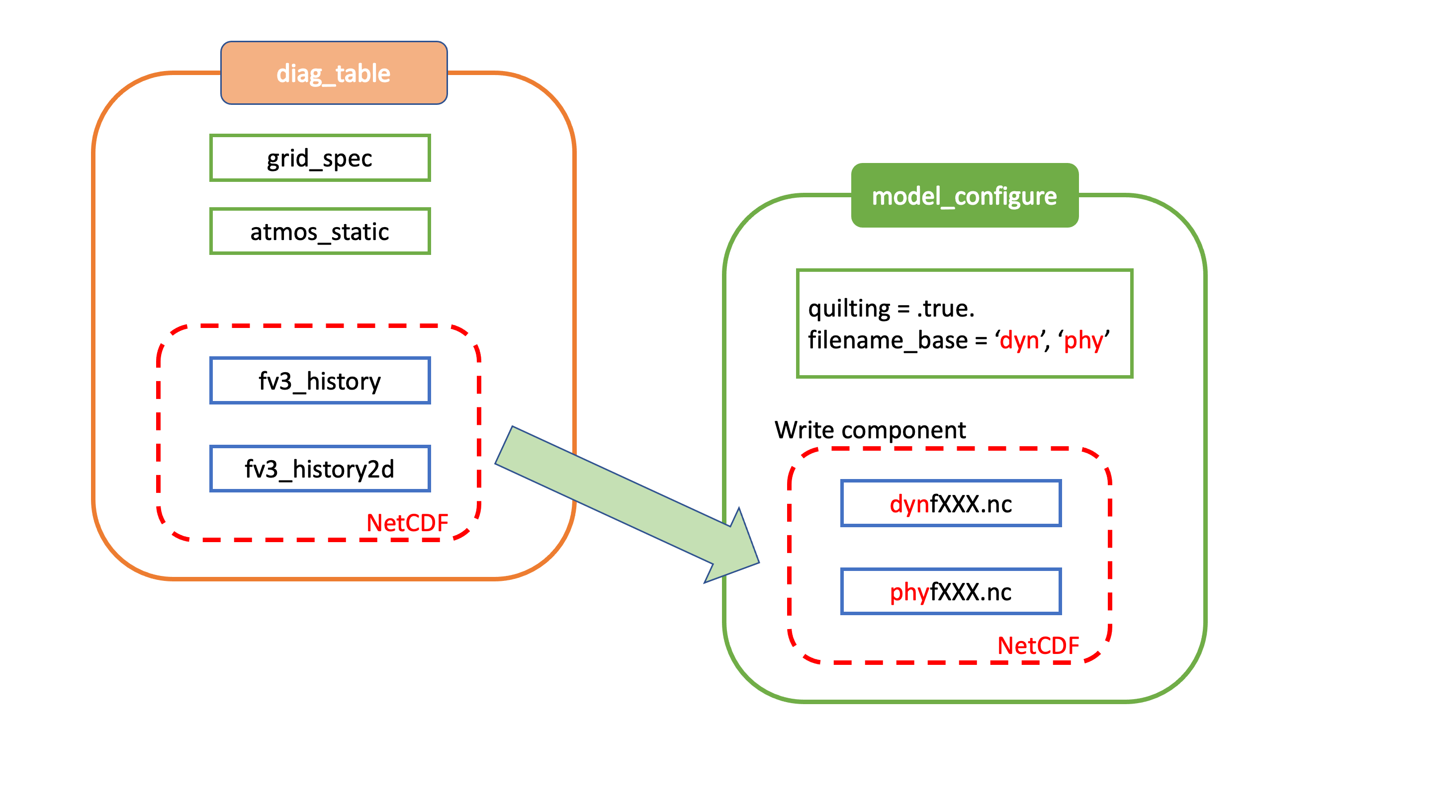
Fig. 4.1 Relationship between diag_table, model_configure and generated output files

Standard output files are logfHHH (one per forecast hour), and out and err as specified by the job submission. ESMF may also produce log files (controlled by variable print_esmf in the model_configure file), called PETnnn.ESMF_LogFile (one per MPI task).

Additional output files include: nemsusage.xml, a timing log file; time_stamp.out, contains the model init time; RESTART/*nc, files needed for restart runs.

4.3.2. MOM6

MOM6 output is controlled via the FMS diag_manager using the diag_table. When MOM6 is present, the diag_table shown above includes additional requested MOM6 fields.

A brief example of the diag_table is shown below. “...” denotes where lines have been removed.

 ######################
 "ocn%4yr%2mo%2dy%2hr",      6,  "hours", 1, "hours", "time", 6, "hours", "1901 1 1 0 0 0"
 "SST%4yr%2mo%2dy",      1,  "days",  1, "days",  "time", 1, "days",  "1901 1 1 0 0 0"
 ##############################################
 # static fields
 "ocean_model", "geolon",      "geolon",      "ocn%4yr%2mo%2dy%2hr", "all", .false., "none", 2
 "ocean_model", "geolat",      "geolat",      "ocn%4yr%2mo%2dy%2hr", "all", .false., "none", 2
 ...
# ocean output TSUV and others
 "ocean_model", "SSH",      "SSH",      "ocn%4yr%2mo%2dy%2hr","all",.true.,"none",2
 "ocean_model", "SST",      "SST",      "ocn%4yr%2mo%2dy%2hr","all",.true.,"none",2
 "ocean_model", "SSS",      "SSS",      "ocn%4yr%2mo%2dy%2hr","all",.true.,"none",2
 ...
# save daily SST
 "ocean_model", "geolon",      "geolon",      "SST%4yr%2mo%2dy", "all", .false., "none", 2
 "ocean_model", "geolat",      "geolat",      "SST%4yr%2mo%2dy", "all", .false., "none", 2
 "ocean_model", "SST",         "sst",         "SST%4yr%2mo%2dy", "all", .true.,  "none", 2

# Z-Space Fields Provided for CMIP6 (CMOR Names):
#===============================================
 "ocean_model_z","uo","uo"      ,"ocn%4yr%2mo%2dy%2hr","all",.true.,"none",2
 "ocean_model_z","vo","vo"      ,"ocn%4yr%2mo%2dy%2hr","all",.true.,"none",2
 "ocean_model_z","so","so"      ,"ocn%4yr%2mo%2dy%2hr","all",.true.,"none",2
 "ocean_model_z","temp","temp"  ,"ocn%4yr%2mo%2dy%2hr","all",.true.,"none",2

# forcing
 "ocean_model", "taux",      "taux",          "ocn%4yr%2mo%2dy%2hr","all",.true.,"none",2
 "ocean_model", "tauy",      "tauy",          "ocn%4yr%2mo%2dy%2hr","all",.true.,"none",2
 ...

4.3.3. HYCOM

HYCOM output configuration is set in the blkdat.input file. A few common configuration options are described in Table 4.29

Table 4.29 The following table describes HYCOM output configuration.

Parameter	Description
dsurfq	Number of days between model diagnostics at the surface
diagfq	Number of days between model diagnostics
meanfq	Number of days between model time averaged diagnostics
rstrfq	Number of days between model restart output
itest	i grid point where detailed diagnostics are desired
jtest	j grid point where detailed diagnostics are desired

HYCOM outpus multiple datasets. These datasets contain both dot-a (.a), dot-b (.b), and dot-txt (.txt) files. Dot-a files contain data written as 32-bit IEEE real values (idm*jdm). Dot-b files contain plain text metadata for each field in the dot-a file. Dot-txt files contain plain text data for a single sell for profiling purposes. Post-processing utilties are available in the HYCOM-tools repository.

Table 4.30 The following table describes HYCOM output files.

Filename	Description
archs.YYYY_DDD_HH.(a,b,txt)	HYCOM surface archive data
archv.YYYY_DDD_HH.(a,b,txt)	HYCOM archive data
restart_out.(a,b)	HYCOM restart files

4.3.4. CICE6

CICE6 output is controlled via the namelist ice_in. The relevant configuration settings are

...
 histfreq       = 'm','d','h','x','x'
 histfreq_n     =  0 , 0 , 6 , 1 , 1
 hist_avg       = .true.
...

In this example, histfreq_n and hist_avg specify that output will be 6-hour means. No monthly (m), daily (d), yearly (x) or per-timestep (x) output will be produced.The hist_avg can also be set .false. to produce, for example, instaneous fields every 6 hours.

The output of any field is set in the appropriate ice_in namelist. For example,

...
&icefields_nml
f_aice         = 'mdhxx'
f_hi           = 'mdhxx'
f_hs           = 'mdhxx'
...

where the ice concentration (aice), ice thickness (hi) and snow thickness (hs) are set to be output on the monthly, daily, hourly, yearly or timestep intervals set by the histfreq_n setting. Since histfreq_n is 0 for both monthly and daily frequencies and neither yearly nor per-timestep output is requested, only 6-hour mean history files will be produced.

Further details of the configuration of CICE model output can be found in the CICE documentation 3.1.4

4.3.5. WW3

The run directory includes WW3 binary outputs for the gridded outputs (YYYYMMDD.HHMMSS.out_grd.<grd>), point outputs (YYYYMMDD.HHMMSS.out_pnt.points) and restart files (YYYYMMDD.HHMMSS.restart.<grd>).

4.3.6. CMEPS

The CMEPS mediator writes general information about the run-time configuration to the file mediator.log in the model run directory. Optionally, the CMEPS mediator can be configured to write history files for the purposes of examining the field exchanges at various points in the model run sequence.

4.4. Additional Information about the FMS Diagnostic Manager

The FMS (Flexible Modeling System) diagnostic manager (FMS/diag_manager) manages the output for the ATM and, if present, the MOM6 component in the UFS Weather Model. It is configured using the diag_table file. Data can be written at any number of sampling and/or averaging intervals specified at run-time. More information about the FMS diagnostic manager can be found at: https://data1.gfdl.noaa.gov/summer-school/Lectures/July16/03_Seth1_DiagManager.pdf

4.4.1. Diagnostic Manager namelist

The diag_manager_nml namelist contains values to control the behavior of the diagnostic manager. Some of the more common namelist options are described in Table 4.31. See FMS/diag_manager/diag_manager.F90 for the complete list.

Table 4.31 Namelist variables used to control the behavior of the diagnostic manager.

Namelist variable	Type	Description	Default value
max_files	INTEGER	Maximum number of files allowed in diag_table	31
max_output_fields	INTEGER	Maximum number of output fields allowed in diag_table	300
max_input_fields	INTEGER	Maximum number of registered fields allowed	300
prepend_date	LOGICAL	Prepend the file start date to the output file. .TRUE. is only supported if the diag_manager_init routine is called with the optional time_init parameter.	.TRUE.
do_diag_field_log	LOGICAL	Write out all registered fields to a log file	.FALSE.
use_cmor	LOGICAL	Override the missing_value to the CMOR value of -1.0e20	.FALSE.
issue_oor_warnings	LOGICAL	Issue a warning if a value passed to diag_manager is outside the given range	.TRUE.
oor_warnings_fatal	LOGICAL	Treat out-of-range errors as FATAL	.FALSE.
debug_diag_manager	LOGICAL	Check if the diag table is set up correctly	.FALSE.

This release of the UFS Weather Model uses the following namelist:

&diag_manager_nml
  prepend_date = .false.
/

4.5. Additional Information about the Write Component

The UFS Weather Model is built using the Earth System Modeling Framework (ESMF). As part of this framework, the output history files written by the model use an ESMF component, referred to as the write component. This model component is configured with settings in the model_configure file, as described in Section 4.2.3. By using the ESMF capabilities, the write component can generate output files in several different formats and several different map projections. For example, a Gaussian global grid in NEMSIO format, or a native grid in NetCDF format. The write component also runs on independent MPI tasks, and so the computational tasks can continue while the write component completes its work asynchronously. The configuration of write component tasks, balanced with compute tasks, is part of the tuning for each specific application of the model (HPC, write frequency, i/o speed, model domain, etc). For the global grid, if the write component is not selected (quilting=.false.), the FV3 code will write tiled output in the native projection in NetCDF format. The regional grid requires the use of the write component.